Ensemble learning is a machine learning technique where multiple models are combined to improve performance. Instead of relying on a single model, ensemble methods leverage the diversity of several models to make more accurate predictions. Common ensemble methods include bagging, boosting, and stacking. Bagging combines multiple models trained on different subsets of the data, boosting sequentially trains models to correct the errors of previous ones, and stacking combines the predictions of multiple models using another model.

Core Concepts
○ Base Learners - Ensemble learning relies on the use of multiple base learners, which can be any machine learning algorithm capable of making predictions. These base learners are trained independently on the same dataset or different subsets of the dataset.
○ Diversity - The effectiveness of ensemble learning depends on the diversity among the base learners. Diversity is achieved by training base learners using different algorithms, different subsets of the training data, or different feature representations. The goal is to ensure that each base learner captures unique patterns or aspects of the data.
○ Aggregation - Once the base learners are trained, their predictions are combined to make the final ensemble prediction. This aggregation can take various forms, such as averaging the predictions (for regression tasks), taking a majority vote (for classification tasks), or using more sophisticated methods like weighted averaging.

Ensemble Methods
○ Bagging (Bootstrap Aggregating) - Bagging involves training multiple base learners independently on random subsets of the training data with replacement. The final prediction is typically obtained by averaging or voting over the predictions of all base learners. Random Forest is a popular example of a bagging ensemble method that uses decision trees as base learners.
○ Boosting - Boosting sequentially trains base learners, with each subsequent learner focusing on the instances that were misclassified by the previous ones. This iterative process allows boosting algorithms to correct errors and improve prediction accuracy over time. AdaBoost (Adaptive Boosting) and Gradient Boosting Machines (GBM) are well-known boosting algorithms.
○ Stacking - Also known as meta-learning, combines the predictions of multiple base learners using another model, called a meta-learner or blender. The base learners' predictions serve as input features for the meta-learner, which learns to generate the final prediction. Stacking can be thought of as a higher-level learning process that learns how to best combine the predictions of the base learners.

Advantages of Ensemble Learning
○ Improved Accuracy - Ensemble methods often achieve higher prediction accuracy than individual base learners by leveraging the strengths of multiple models and mitigating their weaknesses.
○ Robustness - Ensembles are more robust to noisy data and overfitting since they combine predictions from multiple models, reducing the impact of individual errors.
○ Versatility - Ensemble methods are versatile and can be applied to a wide range of machine learning tasks, making them valuable tools in various domains.

Disadvantages of Ensemble Learning
○ Increased Complexity - Ensemble learning typically involves training and combining multiple models, which can significantly increase the computational complexity and resource requirements. Managing and tuning multiple models also adds complexity to the overall machine learning pipeline.
○ Overfitting - While ensemble methods can help reduce overfitting by combining diverse models, there's still a risk of overfitting, especially if the base learners are highly complex or if the ensemble is not properly regularized. Overfitting can occur when the ensemble learns to memorize the noise in the training data rather than capturing the underlying patterns.
○ Dependency on Base Learners - The performance of ensemble learning heavily relies on the quality and diversity of the base learners. If the base learners are poorly chosen or if they exhibit similar behavior, the ensemble may not achieve significant improvements in predictive performance compared to individual models.
○ Training Time - Training an ensemble of models can require more time and computational resources compared to training a single model, particularly if the base learners are complex or if the ensemble size is large. This increased training time may be prohibitive in time-sensitive or resource-constrained environments.

Importance of Ensemble Learning
○ Improved Predictive Performance - By leveraging the strengths of multiple models and combining their predictions, ensemble methods can often achieve higher accuracy and robustness than any individual model.
○ Enhanced Robustness - Ensembles are less sensitive to outliers and noisy data compared to single models. By aggregating predictions from multiple models, ensembles can produce more stable and reliable predictions.
○ Versatility - Ensemble methods are versatile and can be applied to a wide range of machine learning tasks, including classification, regression, anomaly detection, and recommendation systems.

Ensemble Learning Techniques:

1. Bagging (Bootstrap Aggregating)
Core Concepts
○ Bootstrap Sampling - Bagging begins by randomly selecting multiple bootstrap samples from the original training dataset. Bootstrap sampling involves randomly selecting data points from the original dataset with replacement, resulting in multiple subsets of the data with the same size as the original dataset. Each bootstrap sample is used to train a separate base learner.
○ Base Learners - Bagging employs multiple base learners, which can be any machine learning algorithm capable of making predictions. Each base learner is trained independently on one of the bootstrap samples, resulting in a diverse set of models that capture different aspects of the data.
○ Aggregation - Once the base learners are trained, their predictions are combined using aggregation methods such as averaging (for regression tasks) or voting (for classification tasks). The final prediction is typically obtained by aggregating the predictions of all base learners.

Applications of Bagging
○ Random Forest - One of the most well-known implementations of bagging is the Random Forest algorithm. Random Forest builds an ensemble of decision trees, where each tree is trained on a random subset of features and a bootstrap sample of the training data. By aggregating the predictions of multiple decision trees, Random Forest achieves high prediction accuracy and robustness in various machine learning tasks, including classification and regression.
○ Ensemble of Different Base Learners - Bagging can also be applied to ensembles consisting of different types of base learners, such as support vector machines, neural networks, or k-nearest neighbors. By combining predictions from diverse models, bagging can further enhance the performance and robustness of the ensemble across different types of machine learning problems.

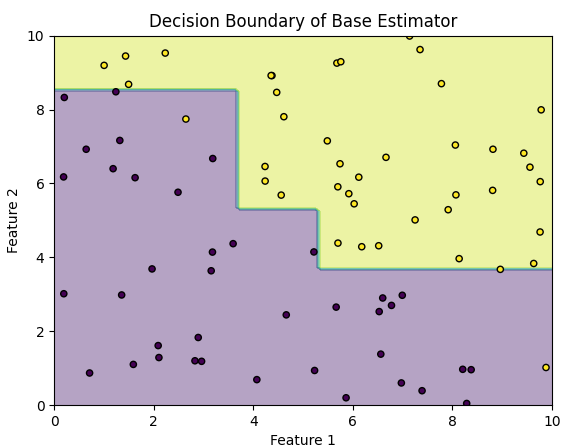
Code example - The below code generates random data points in a 2-dimensional space and assigns labels based on a simple decision boundary. It then uses a Bagging classifier with decision trees as base estimators to classify the data and visualize the decision boundary of one of the base estimators.

 import numpy as np
 import matplotlib.pyplot as plt
 from sklearn.ensemble import BaggingClassifier
 from sklearn.tree import DecisionTreeClassifier
 from sklearn.metrics import accuracy_score
                            
 # Generate synthetic data
 np.random.seed(0)
 X = np.random.rand(100, 2) * 10
 y = (X[:, 0] + X[:, 1] > 10).astype(int)
                            
 # Splitting the data into training and testing sets
 X_train, X_test = X[:80], X[80:]
 y_train, y_test = y[:80], y[80:]
                            
 # Define base classifier
 base_classifier = DecisionTreeClassifier()
                            
 # Initialize Bagging classifier
 bagging_classifier = BaggingClassifier(base_classifier, n_estimators=10, random_state=42)
                            
 # Train Bagging classifier
 bagging_classifier.fit(X_train, y_train)
                            
 # Predict
 y_pred = bagging_classifier.predict(X_test)
                            
 # Calculate accuracy
 accuracy = accuracy_score(y_test, y_pred)
 print("Accuracy:", accuracy)
                            
 # Plot decision boundary for one base estimator
 base_estimator = bagging_classifier.estimators_[0]
 xx, yy = np.meshgrid(np.linspace(0, 10, 100), np.linspace(0, 10, 100))
 Z = base_estimator.predict(np.c_[xx.ravel(), yy.ravel()])
 Z = Z.reshape(xx.shape)
                            
 plt.contourf(xx, yy, Z, alpha=0.4)
 plt.scatter(X_train[:, 0], X_train[:, 1], c=y_train, s=20, edgecolor='k')
 plt.xlabel('Feature 1')
 plt.ylabel('Feature 2')
 plt.title('Decision Boundary of Base Estimator')
 plt.show()
                            

2. Boosting
Core Concepts
○ Sequential Training - Unlike bagging, where base learners are trained independently, boosting sequentially trains base learners in a stage-wise fashion. Each base learner is trained to focus on the instances that were misclassified by the previous ones, thereby gradually improving the ensemble's performance.
○ Focus on Misclassified Instances - Boosting assigns higher weights to instances that were misclassified by previous base learners, effectively directing subsequent learners' attention towards these challenging instances. By iteratively focusing on the most difficult examples, boosting can progressively reduce the training error and improve generalization.
○ Weighted Aggregation - In boosting, the predictions of base learners are combined using weighted aggregation, where more weight is given to the predictions of base learners with lower training error. This weighted combination ensures that base learners with better performance contribute more to the final prediction.

Applications of Boosting
○ AdaBoost (Adaptive Boosting) - One of the earliest and most popular boosting algorithms. It assigns higher weights to misclassified instances and adjusts the weights of base learners based on their performance. AdaBoost is widely used in binary classification tasks and has been successfully applied to various domains, including face detection and spam filtering.
○ Gradient Boosting Machines (GBM) - Gradient Boosting Machines sequentially train base learners by minimizing a loss function with gradient descent. GBM is a powerful and flexible boosting algorithm that can handle various types of data and loss functions.

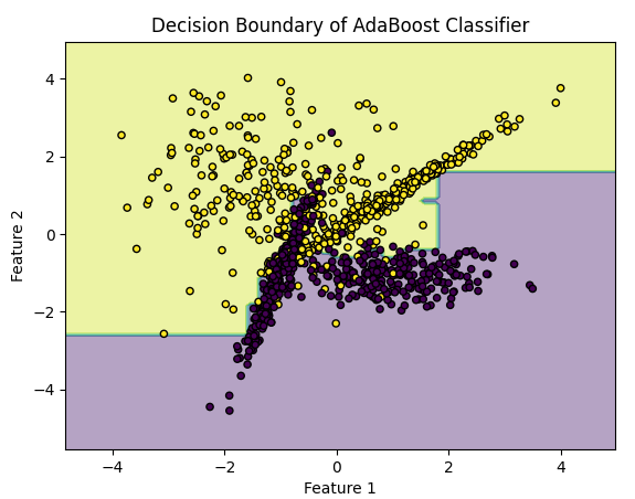
Code example - The brlow code generates a synthetic dataset with two features, splits it into training and testing sets, creates an AdaBoost classifier with decision trees as weak learners, trains the AdaBoost classifier, predicts on the test set, calculates accuracy, and plots the decision boundary of the AdaBoost classifier.

 import numpy as np
 import matplotlib.pyplot as plt
 from sklearn.datasets import make_classification
 from sklearn.model_selection import train_test_split
 from sklearn.ensemble import AdaBoostClassifier
 from sklearn.tree import DecisionTreeClassifier
 from sklearn.metrics import accuracy_score
        
 # Generate synthetic dataset
 X, y = make_classification(n_samples=1000, n_features=2, n_informative=2, n_redundant=0, n_classes=2, random_state=42)
 
 # Split dataset into training and testing sets
 X_train, X_test, y_train, y_test = train_test_split(X, y, test_size=0.2, random_state=42)
 
 # Define base classifier
 base_classifier = DecisionTreeClassifier(max_depth=1)
        
 # Initialize AdaBoost classifier
 adaboost_classifier = AdaBoostClassifier(base_classifier, n_estimators=50, learning_rate=1, random_state=42)
 
 # Train AdaBoost classifier
 adaboost_classifier.fit(X_train, y_train)
        
 # Predict
 y_pred = adaboost_classifier.predict(X_test)
        
 # Calculate accuracy
 accuracy = accuracy_score(y_test, y_pred)
 print("Accuracy:", accuracy)
        
 # Plot decision boundary
 x_min, x_max = X[:, 0].min() - 1, X[:, 0].max() + 1
 y_min, y_max = X[:, 1].min() - 1, X[:, 1].max() + 1
 xx, yy = np.meshgrid(np.arange(x_min, x_max, 0.1), np.arange(y_min, y_max, 0.1))
 Z = adaboost_classifier.predict(np.c_[xx.ravel(), yy.ravel()])
 Z = Z.reshape(xx.shape)
        
 plt.contourf(xx, yy, Z, alpha=0.4)
 plt.scatter(X[:, 0], X[:, 1], c=y, s=20, edgecolor='k')
 plt.xlabel('Feature 1')
 plt.ylabel('Feature 2')
 plt.title('Decision Boundary of AdaBoost Classifier')
 plt.show()
                            

3. Stacking (Stacked Generalization)
Core Concepts
○ Base Learners - Stacking begins by training a set of diverse base learners, each of which may use different algorithms or modeling techniques. These base learners independently make predictions on the training data.
○ Meta-Learner - Once the base learners have made their predictions, a meta-learner is trained on the base learners' predictions as features, along with the original input features. The meta-learner learns to combine the predictions of the base learners in a way that optimizes the overall predictive performance.
○ Hierarchical Structure - Stacking introduces a hierarchical structure to the ensemble, where base learners make predictions at the first level, and the meta-learner makes the final prediction at the second level. This hierarchical approach allows stacking to capture complex interactions between the base learners' predictions and the input features.

Applications of Stacking
○ Model Fusion - Stacking is commonly used in machine learning competitions, where participants combine multiple diverse models to achieve the best predictive performance. By fusing the predictions of different models using a meta-learner, stacking can effectively blend the strengths of individual models and produce more accurate predictions.
○ Feature Engineering - Stacking can also be used for feature engineering by incorporating meta-features derived from the predictions of base learners. These meta-features can capture valuable information about the data distribution and help improve predictive performance.

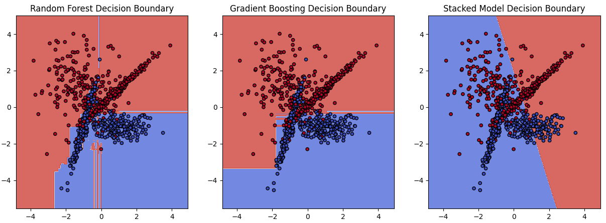
Code example - The below example uses a RandomForestClassifier and a GradientBoostingClassifier as base models, and a LogisticRegression as the meta-model. We're generating a synthetic dataset with 1000 samples, 2 features, and 2 classes. We're also specifying that only 2 of the features should be informative, and that there should be no redundant or repeated features.

 import numpy as np
 import matplotlib.pyplot as plt
 from sklearn.datasets import make_classification
 from sklearn.model_selection import train_test_split
 from sklearn.ensemble import RandomForestClassifier, GradientBoostingClassifier
 from sklearn.linear_model import LogisticRegression
 from sklearn.metrics import accuracy_score
        
 # Generate synthetic dataset with 2 features
 X, y = make_classification(n_samples=1000, n_features=2, n_classes=2, n_informative=2, n_redundant=0, n_repeated=0, random_state=42)
        
 # Split dataset into training and testing sets
 X_train, X_test, y_train, y_test = train_test_split(X, y, test_size=0.2, random_state=42)
        
 # Base models
 base_model1 = RandomForestClassifier(n_estimators=50, random_state=42)
 base_model2 = GradientBoostingClassifier(n_estimators=50, random_state=42)
        
 # Meta model
 meta_model = LogisticRegression()
        
 # Train base models
 base_model1.fit(X_train, y_train)
 base_model2.fit(X_train, y_train)
        
 # Generate predictions from base models
 pred1 = base_model1.predict(X_train)
 pred2 = base_model2.predict(X_train)
        
 # Stack predictions horizontally
 stacked_predictions_train = np.column_stack((pred1, pred2))
        
 # Train meta model on stacked predictions
 meta_model.fit(stacked_predictions_train, y_train)
        
 # Generate predictions from base models for test set
 pred1_test = base_model1.predict(X_test)
 pred2_test = base_model2.predict(X_test)
        
 # Stack predictions horizontally for test set
 stacked_predictions_test = np.column_stack((pred1_test, pred2_test))
        
 # Make final prediction using meta model
 final_pred = meta_model.predict(stacked_predictions_test)
        
 # Calculate accuracy
 accuracy = accuracy_score(y_test, final_pred)
 print("Accuracy:", accuracy)
        
 # Plot decision boundaries of base models
 def plot_decision_boundary(ax, clf, X, y):
    h = .02  # step size in the mesh
    x_min, x_max = X[:, 0].min() - 1, X[:, 0].max() + 1
    y_min, y_max = X[:, 1].min() - 1, X[:, 1].max() + 1
    xx, yy = np.meshgrid(np.arange(x_min, x_max, h),
        np.arange(y_min, y_max, h))
    Z = clf.predict(np.c_[xx.ravel(), yy.ravel()])
    Z = Z.reshape(xx.shape)
    ax.contourf(xx, yy, Z, cmap=plt.cm.coolwarm, alpha=0.8)
    ax.scatter(X[:, 0], X[:, 1], c=y, cmap=plt.cm.coolwarm, s=20, edgecolors='k')
        
 # Plot decision boundaries of base models
 fig, axs = plt.subplots(1, 3, figsize=(15, 5))
        
 # Plot decision boundaries of base model 1
 axs[0].set_title('Random Forest Decision Boundary')
 plot_decision_boundary(axs[0], base_model1, X_train, y_train)
        
 # Plot decision boundaries of base model 2
 axs[1].set_title('Gradient Boosting Decision Boundary')
 plot_decision_boundary(axs[1], base_model2, X_train, y_train)
        
 # Plot decision boundaries of stacked model
 axs[2].set_title('Stacked Model Decision Boundary')
 plot_decision_boundary(axs[2], meta_model, X_train, y_train)
        
 plt.show()
                            

Ensemble Learning in Practice
Ensemble learning techniques have found widespread use in various real-world applications across different domains due to their ability to improve predictive performance, robustness, and generalization. In practice, ensemble learning involves several key steps, including data preprocessing, model selection, ensemble construction, and evaluation.

Data Preprocessing - Before applying ensemble learning techniques, it's essential to preprocess the data to ensure it's clean, normalized, and appropriately formatted. Data preprocessing steps may include:
○ Handling missing values
○ Feature scaling or normalization
○ Encoding categorical variables
○ Feature selection or dimensionality reduction
○ Handling imbalanced datasets

Model Selection - The choice of base learners plays a crucial role in the success of ensemble learning. Practitioners typically experiment with a variety of machine learning algorithms and model architectures to build a diverse set of base learners. Some common base learners used in ensemble learning include:
○ Decision trees (e.g., Random Forest, Gradient Boosting Machines)
○ Support Vector Machines
○ Neural networks (e.g., deep learning models)
○ k-Nearest Neighbors
○ Linear models (e.g., Logistic Regression)

Ensemble Construction - Once the base learners are chosen, they are trained on the training data to make predictions. The ensemble construction process varies depending on the ensemble technique used:
○ Bagging
○ Boosting
○ Stacking

Evaluation - Once the ensemble model is constructed, it is evaluated on a separate validation or test dataset to assess its performance. Common evaluation metrics include accuracy, precision, recall, F1-score, area under the ROC curve (AUC), mean squared error (MSE), and others, depending on the nature of the problem.

Real-world applications of ensemble learning
Ensemble learning techniques have been successfully employed in numerous real-world scenarios across diverse domains, including finance, healthcare, e-commerce, image and speech recognition, natural language processing, and more.

1. Finance
○ Stock Market Prediction - Ensemble methods are used to forecast stock prices by combining predictions from multiple models trained on historical stock data, economic indicators, and news sentiment analysis.
○ Credit Risk Assessment - Ensemble models help financial institutions assess the creditworthiness of borrowers by combining information from multiple sources, such as credit scores, income, and repayment history.
○ Fraud Detection - Ensemble learning techniques are utilized to detect fraudulent transactions by aggregating predictions from different fraud detection models based on transactional patterns and anomaly detection.

2. Healthcare
○ Disease Diagnosis - Ensemble models assist healthcare professionals in diagnosing diseases such as cancer, diabetes, and cardiovascular disorders by integrating information from medical tests, imaging scans, and patient records.
○ Patient Outcome Prediction - Ensemble learning is employed to predict patient outcomes, including mortality risk, hospital readmission, and treatment response, based on clinical data and electronic health records.
○ Drug Discovery - Ensemble methods aid in drug discovery and development by predicting the efficacy and safety of potential drug candidates using molecular structure data and biological assays.

3. E-commerce
○ Customer Churn Prediction - Ensemble models help e-commerce companies predict customer churn by combining information from transaction histories, website interactions, and customer demographics to identify at-risk customers.
○ Recommendation Systems - Ensemble learning techniques power recommendation systems by aggregating predictions from multiple recommendation algorithms to personalize product recommendations for users based on their preferences and behavior.
○ Personalized Marketing - Ensemble models enable targeted marketing campaigns by combining insights from customer segmentation, purchase history, and demographic data to deliver personalized offers and promotions.
4. Image and Speech Recognition
○ Object Detection - Ensemble methods are used for object detection in images and videos, where multiple object detection models are combined to accurately identify and localize objects of interest.
○ Facial Recognition - Ensemble learning techniques enhance facial recognition systems by integrating predictions from multiple face recognition algorithms to improve accuracy and robustness in identifying individuals.
○ Speech Recognition - Ensemble models aid in speech recognition tasks by combining predictions from multiple speech recognition engines to transcribe spoken language into text with higher accuracy.

5. Natural Language Processing (NLP)
○ Sentiment Analysis - Ensemble learning is applied to sentiment analysis tasks, where predictions from multiple sentiment analysis models are combined to analyze and classify opinions expressed in text data, such as social media posts and product reviews.
○ Text Classification - Ensemble methods assist in text classification tasks, including topic classification, spam detection, and language identification, by aggregating predictions from diverse classification models.
○ Machine Translation - Ensemble models improve machine translation systems by combining outputs from multiple translation models to generate more accurate translations across different languages.

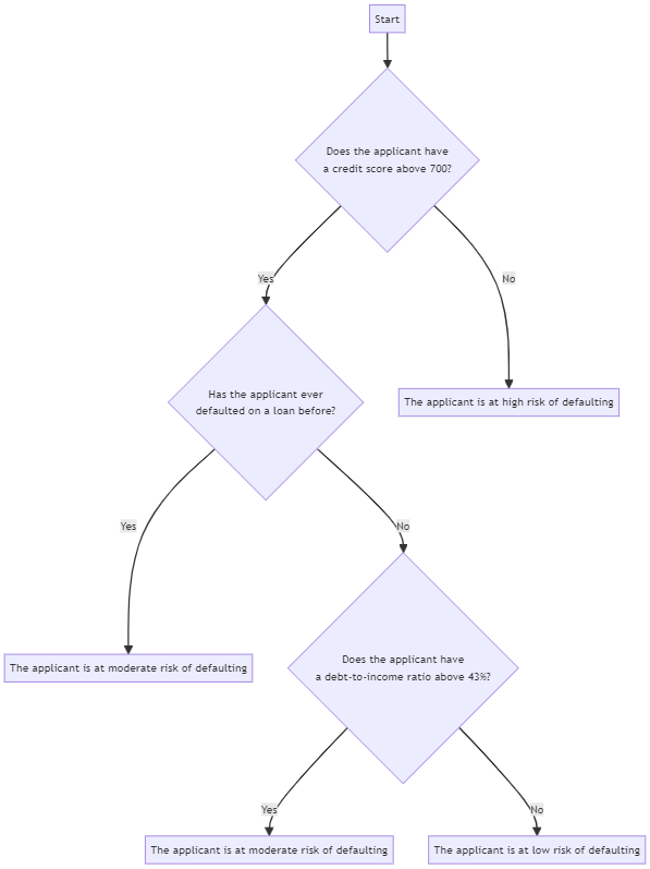
The below diagram illustrates a basic example of Credit Risk Assessment.

Ensemble learning is a versatile and powerful machine learning technique that combines the predictions of multiple models to improve predictive performance, robustness, and generalization. It continues to be a valuable tool in machine learning and data science, offering a powerful approach to improving predictive performance and addressing complex real-world challenges.

You might also like: